0. Introduction Recursion is a pervasive problem-solving tool both in mathematics and in computer science. In both realms we have a basic process that launches a similar process on a similar subsystem.
We will demostrate its use in two realms: geometry and combinatorics. We will begin by doing a scissors and paper construction of a Sierpinski tetrahedron. We will then analyze the behavior of the volume and surface area as the number of iterations gets large. We will use simple recursion to write down formulae for these quantities. This workshop is held in a lab containing computers loaded with Python; participants get a chance to try it out themselves.
In the second part, we will look at recursion as a tool for solving combinatorial problems. and we will use recursion to compute some geometric quantities associated with the Sierpinski tetrahedron construction we conduct here. We will introduce the essentials of the Python language necessary to facilitate these computations. We will look at this problem: If a group of people contains n members, in how many ways can we divide it into k subcomittees?. If time permits we wil show several other applications of recursion.
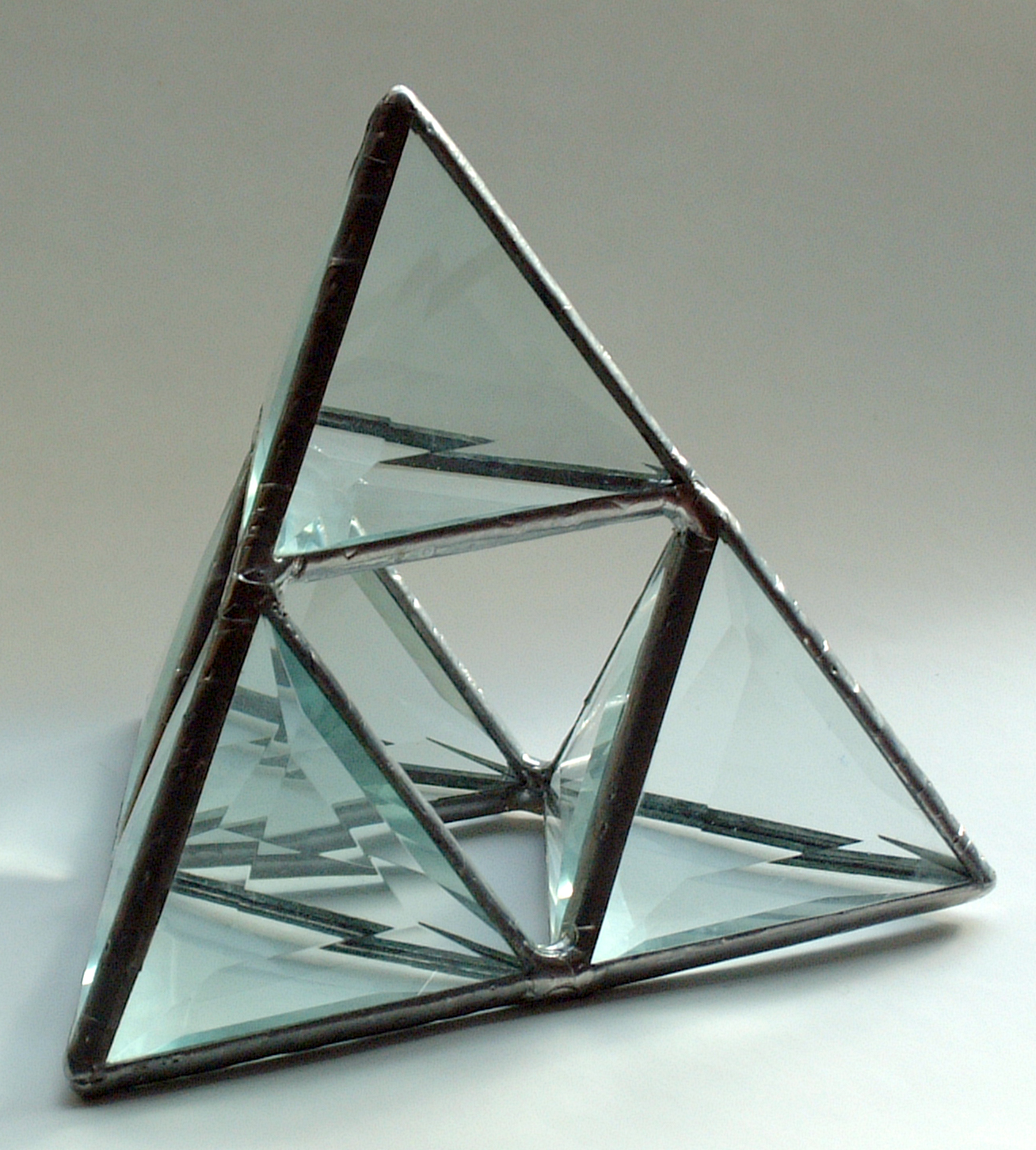
1. The Sierpinski Construction Suppose you have a regular tetrahedron; let us denote its initial volume by V(0) and its initial surface area by A(0). Along each edge, mark off the midpoint. This defines four child tetrahedrons as is illustrated in the model below.
Each succeeding step repeats this procedure on each of the child tetrahedrons of its predecessor. Pictured here is the second step in the process.
Now that you have seen this and understand the progression, we will develop an analysis of the surface area and the volume of the object created after n steps.
To do this, let us analyze the effect of performing one step of the construction.
First let us deal with surface area. On each face, we remove one-quarter of the area, so the outer surface loses one-quarter of its area. However, if you look at the inside, you will see four new surfaces are created whose area equals the four surfaces we just excised. As a result, A(1) = A(0). Recursivlely the subsequent step has the same effect on each of its child tetrahedrons; we have A(n) = A(n-1) for all n. The surface area remains constant.
Next we look at the volume. Each time we do the construction the number of tetrahedrons increases by a factor of 4. Since each child tetrahedron has all of its dimenions halved in the construction from its parent, the volume of the each child is 1/8 that of the parent. As a result, we lose half the volume on each iteraton: A(n + 1) = A(n)/2 for n ≥ 0.
As a result, we have A(n) = A(0) and V(n) = V(0)*2-n, for n ≥ 0.
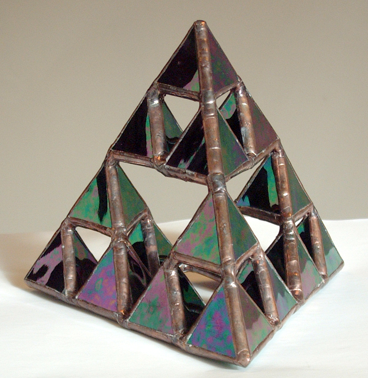
Pictured below are the objects created by each group.

2. Python Preliminaries Python is an open-source scripting language that is available for free on your favorite computing platform. The syntax is simple and its organization seems to be very appealing to mathematicians, owing it its functional organization. It is a small program that runs on even fairly outmoded machines. Every student can have it at home for free, and it can be loaded on all machines in a school with no worry about licensing. You can obtain Python and lots of tutorials and documentation from www.python.org. A succinct introduction is posted on Morrison's page; this is his 2005 TCM talk.
We will give a very bare-bones introduction to Python sufficient for our purposes today. Python variables are brought into existence when you initialize them. Here is an example
x = 5
stores the value 5 in the location x. Notice that there is no "type" declaration, since objects in Python are dyanamically typed. This is just like storing the number 5 in register x on your TI calculator.
We define a function in Python as follows.
def f(x):
	return x*x
Call this function by typing something like
f(5.5)
Python will inform you that f(5.5) = 30.25.
The variables you create in various functions are separate from each other; you don't need to worry excessively about "running out of names".
A function in Python can have several variables; here is an example
def cow(x, y):
	if x < y:
		return x #return ends execution of a function
	return y  #Here iss how we return the output otherwise.
This function returns the minimum of x and y. To invoke it in Python, just type
cow(??, ???)
In computing, functions behave a little differently then their mathematical counterparts. Functions can have zero or more inputs, and they have one output, just as in the mathematical world. However, they can also have "side effects", such as printing information to the screen.
Here are two examples.
def hi():
	print "Hi!"  #no input, no output, only side effect
This function is "pure side effect" and no input; it simply orders Python to put "Hi!" to the screen.
def greet(name):
	print "Hello, " + name
This function is pure side effect with one input.
For more particulars on Python that will bring you quickly up to speed, see Morrison's Home Page, and select his TCM2005 talk from the navigation menu. You can see it also by hitting this link
3. Recursion Recursive functions are functions that call themselves. Consider this example
def houston(n)
	if n == 0:
		print "Blastoff"
	else:
		print n
		houston(n - 1)
The call houston(5) lets loose the following sequence of events. Since 5 is not zero,
houston(5)begets
print 5 (5 gets put to the screen on its own line)
houston(4)
which begets
print 4 (4 gets printed on its own line)
houston(3)
which begets
print 3 (3 gets printed on its own line)
houston(2)
which begets
print 2 (2 gets printed on its own line)
houston(1)
print 1 (1 gets printed on its own line)
Blastoff!  # this is houston(0) at work.
The call's output is
5
4
3
2
1
Blastoff!!
Python can be used to compute binomal coefficients in a simple way. Let us denote by b(n,k) the number of subsets of size k in a set of size n. We are all familiar with the Pascal Triangle identity
b(n,k) = b(n-1,k-1) + b(n-1,k)and
b(n,0) = b(n,n) = 1, if n >=0
b(n,k) = 0 if k < 0 or k > n
Here is an quick way to compute binomial coefficients without factorials. Unfortunately, whilst the solution is elegant, it it also exhibits elephantine inefficiency.
def bin(n):
	if k == 0 or k == n:
		return 1
	if k < 0 or k > n:
		return 0
	else
		return bin(n-1, k-1) + bin(n-1,k)
4. The Partition Problem How do you compute the number of ways to partition a set of size n into k nonvoid subsets? We will provide a recursive solution here. We will denote this quantity by part(n,k). Let us begin by ferreting out the "obvious" cases. Let k = 1. If n is a positive integer, there is one partition of the n elements of an set of size n into n subsets (Each must have size 1!); hence part(n,n) = 1 for all positive integers n. How about p(n,1)? It is even easier to see that part(n,1) = 1 for all positive integers n.
Now suppose we have a set of size n. Let us fix an element and denote it by 1. Now let's look at the remaining n - 1 elements. Partition these into k subsets: there are part(n-1, k -1) ways to do this. Now we will throw the element 1 into one of these subsets: there are k ways to do this. This is the way we can build all the partitions in which 1 is not by itself. There are k*part(n-1,k-1) such partitions.
Remaining are all the partitions which keep 1 all by itself. To get these, first sequester 1 all by itself. That uses up one of the k subsets in the partition. We have k-1 subsets left and n-1 elements to broadcast amongst them. This can be done part(n-1,k-1) ways.
We conclude that
part(n,k) = part(n-1,k-1) + k*part(n-1,k).
With this formula in hand the rest is easy.
def part(n,k):
	if k < n or k > n:
		return 0
	if k == 0 or k == n:
		return 1
	return part(n -1, k -1) + k*part(n-1, k)
5. Conclusion The problems of the partition problem and that of analyzing the Sierpinski construction on the tetrahedron at first appear quite disparate. However, we see that these problems conceptually united by the technique used to solve them: recursion. Recursion allows us to look "one deep at a time" at a probem and arrive at its ultimate solution in an elegant and simple manner.
Epilogue: Assorted Code Examples
Here is an efficient way to compute powers, especially for decimal numbers. The print statement is to illustrate how few times the function calls itself, even to compute a high power. To compute an nth power, about log2(n) calls are made. This is a good use of recursion.
def power(z, n):
    print "called power"
    if n == 0:
        return 1
    if n % 2 == 0:
        return power(z*z, n/2)
    if n % 2 == 1:
        return power(z*z, n/2)*z
Python has an array (list facility). Here is a nice way to sum a list of numbers without looping.
def addme(x):
	s = 0
	if len(s) == 0:
		return 0
	return x[0] + addme(x[1:])  (sum first element + rest of list)
You can also do this to compute sum(a(k), k = 1..n).
def a(n):
	return n*n
	#put whatever function of n you want in here; I put n*n
def add(n):
	if n == 0:
		return a(0)
	return add(n-1) + a(n)
Here is an example of a bad use of recursion.
def fibonacci(n):
	if n == 0 or n == 1:
		return n
	return fibonacci(n-1) + fibonacci(n-2)
Why bad? Each function call begets two new calls. During execution, the number of calls mushrooms to a huge size then collapses.